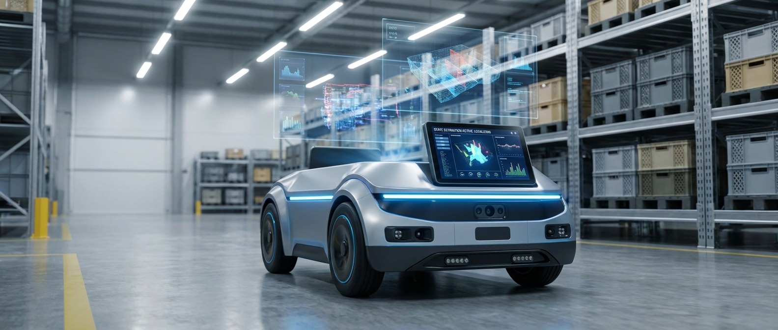
State Estimation
The mathematical backbone of autonomous navigation that allows AGVs to determine "where am I?" in real-time. By fusing noisy sensor data with control inputs, state estimation provides the precise position, orientation, and velocity required for safe operation.
Core Concepts
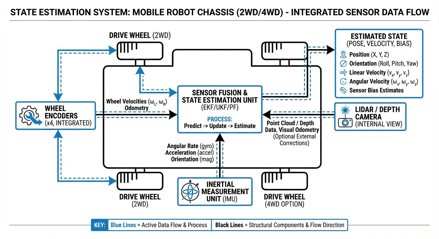
Sensor Fusion
The process of combining data from disparate sources (IMU, wheel encoders, LiDAR) to reduce uncertainty. The aggregate result is more accurate than any single sensor could provide alone.
Probabilistic Modeling
Robots never know their state with 100% certainty. We model position as a probability distribution (Gaussian), allowing the system to make safe decisions even with noisy data.
Odometry (Dead Reckoning)
Estimating position change by measuring wheel rotation. While precise over short distances, it suffers from "drift" over time due to wheel slippage and requires correction.
The Kalman Filter
The industry-standard algorithm for linear state estimation. It operates in a two-step cycle: "Predict" (where we think we moved) and "Update" (what sensors actually saw).
Pose (6 Degrees of Freedom)
The complete state includes position (X, Y, Z) and orientation (Roll, Pitch, Yaw). For standard warehouse AGVs, we typically focus on X, Y, and Yaw (2D Pose).
Loop Closure
The ability of the robot to recognize a location it has visited before. This event triggers a global optimization that corrects accumulated drift errors in the estimated path.
How It Works: The Prediction-Correction Cycle
State estimation is a continuous loop that runs hundreds of times per second. It begins with Prediction, where the robot uses its control inputs (e.g., "I commanded the motors to move 1 meter/second") to guess its new location.
Simultaneously, the Correction phase ingests real-world data from LiDAR, cameras, or GPS. If the LiDAR sees a wall 2 meters away, but the prediction thought it was 2.5 meters away, the algorithm calculates a weighted average based on the reliability (covariance) of each source.
The result is a highly accurate estimate that is better than either the wheel encoders or the external sensors could produce individually, ensuring the AGV navigates tight corridors without collisions.
Real-World Applications
High-Throughput Warehousing
AMRs rely on precise state estimation to navigate dynamic environments with human traffic. Accurate localization allows for tighter packing of inventory shelves and narrower aisles.
Precision Manufacturing
In automotive assembly, AGVs must dock with conveyors with millimeter-level accuracy. Multi-sensor fusion ensures the vehicle aligns perfectly to transfer heavy loads safely.
Outdoor Logistics
When moving between buildings, robots lose LiDAR reflectivity and must rely on GPS/IMU fusion. State estimation algorithms handle the transition between indoor (SLAM) and outdoor navigation seamlessy.
Healthcare Delivery
Hospital robots operate in corridors with glass walls and uniform features. Advanced estimation filters out reflection noise to ensure medication is delivered to the correct room every time.
Frequently Asked Questions
What is the difference between Odometry and State Estimation?
Odometry is a specific type of dead reckoning that uses wheel encoders to estimate position change. State Estimation is the broader framework that takes odometry as just one input and combines it with other sensors (LiDAR, IMU) to correct the inevitable errors and drift that occur in raw odometry.
Why can't we just use GPS for robot localization?
Standard GPS typically has an accuracy of 2-5 meters, which is insufficient for navigating warehouse aisles or doorways. Furthermore, GPS signals are blocked indoors, necessitating local state estimation methods using LiDAR or cameras.
What is the "Hidden Markov Model" assumption in robotics?
This is the assumption that the robot's future state depends only on its current state and the action it takes right now, not on its entire history. This assumption drastically simplifies the mathematics, allowing state estimation algorithms to run in real-time on onboard computers.
Kalman Filter vs. Particle Filter: Which is better?
The Kalman Filter (specifically EKF) is computationally efficient and great for systems with Gaussian noise, making it standard for velocity and continuous tracking. Particle Filters are more computationally intensive but better at "global localization" (figuring out where you are when completely lost) because they can track multiple hypotheses simultaneously.
How does wheel slip affect state estimation?
Wheel slip causes the encoders to register movement that didn't physically happen, leading to significant odometry errors. A robust state estimator detects this discrepancy by cross-referencing with the IMU (which detects acceleration) or visual data, effectively "trusting" the encoders less during slippery conditions.
What role does the IMU (Inertial Measurement Unit) play?
The IMU provides high-frequency data on acceleration and rotational velocity. It is critical for "short-term" estimation, filling in the gaps between slower LiDAR or camera updates, and provides the best data regarding the robot's orientation (pitch/roll).
What is covariance matrix and why does it matter?
The covariance matrix represents the "uncertainty" or confidence of the state estimate. It tells the robot not just "you are at X,Y," but "you are likely within this circle around X,Y." As the robot moves without external correction, this uncertainty grows.
How does State Estimation relate to SLAM?
SLAM (Simultaneous Localization and Mapping) is a complex extension of state estimation. While state estimation assumes a known map to find position, SLAM tries to build the map and find the position within it at the same time.
What happens in a "Kidnapped Robot" scenario?
This occurs when a robot is physically picked up and moved. Standard Kalman filters often fail here because the jump is non-linear. To recover, the system usually requires a global relocalization routine, often triggered by a Particle Filter or visual feature matching.
Is 3D State Estimation necessary for flat warehouses?
Generally, no. For AGVs on flat concrete, we simplify the problem to 2D (x, y, yaw). However, if the robot navigates ramps or uneven terrain, full 6-DOF (Degree of Freedom) estimation becomes necessary to prevent orientation errors from corrupting position data.
How computationally expensive is this process?
Basic EKF (Extended Kalman Filter) is very lightweight and runs easily on microcontrollers. However, heavy sensor processing (like processing 3D Point Clouds from LiDAR for scan matching) to feed the filter requires more powerful CPUs or GPUs found on modern AMRs.
How do dynamic obstacles (people, forklifts) affect estimation?
Dynamic obstacles can confuse LiDAR-based estimation if they block the view of static map features (walls). Advanced algorithms filter out moving points from the scan data before using them for localization to maintain accuracy in busy environments.