Jacobian Matrix
The mathematical bridge that translates individual wheel velocities into precise robot motion. Essential for developing smooth path-planning algorithms and kinematic control for modern AGV fleets.

Core Concepts
Velocity Mapping
Maps the relationship between joint space (wheel rotations) and Cartesian space (linear/angular velocity of the chassis) instantaneously.
The Inverse Jacobian
Critical for control loops. By inverting the matrix ($J^{-1}$), we calculate the required motor speeds to achieve a desired robot trajectory.
Singularity Analysis
Identifies configurations where the robot loses a degree of freedom. In mobile manipulation, avoiding these states prevents loss of control.
Static Force Transmission
Using the principle of virtual work, the Jacobian Transpose maps external forces acting on the chassis back to required motor torques.
Non-Holonomic Constraints
For differential drive AGVs, the Jacobian encodes constraints (like the inability to move sideways), restricting the actionable null space.
Mecanum Drive Matrix
In omnidirectional robots, the Jacobian is fully rank-sufficient, allowing simultaneous translation in X/Y and rotation in Theta.
How It Works
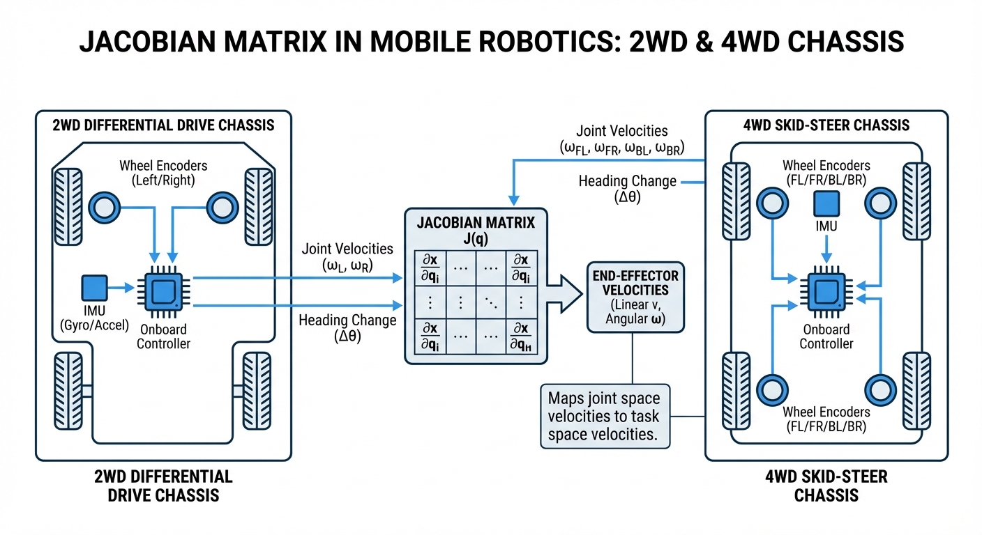
The Jacobian matrix ($J$) acts as a linear transformation operator. In the context of a differential drive AGV, it relates the angular velocities of the left and right wheels ($\dot{\phi}_L, \dot{\phi}_R$) to the linear velocity ($v$) and angular velocity ($\omega$) of the robot center.
Mathematically, the equation takes the form $\dot{x} = J \cdot \dot{q}$. Here, $\dot{x}$ represents the task space vector (how fast the robot moves in the world), and $\dot{q}$ represents the configuration space vector (how fast the wheels spin).
By constantly solving this equation in real-time control loops (typically 50Hz to 1000Hz), the robot controller ensures that the physical wheel hardware strictly adheres to the path planned by the navigation software, compensating for geometry and kinematic constraints.
Real-World Applications
Precision Docking
AGVs require sub-millimeter accuracy when docking with conveyors or charging stations. The Jacobian allows for micro-adjustments in wheel speed to align the chassis perfectly with external markers.
Mobile Manipulation
For robots with arms mounted on mobile bases, a "Whole Body Jacobian" couples the base kinematics with the arm kinematics, allowing the arm to reach for objects while the base is still moving.
Omnidirectional Navigation
In warehousing robots using Mecanum wheels, the Jacobian matrix is 3x4 (for 4 wheels). It enables complex maneuvers like strafing sideways into narrow aisles without rotating the chassis.
Dynamic Obstacle Avoidance
When a person steps in front of an AGV, the local planner generates a new velocity vector. The Inverse Jacobian instantly translates this escape vector into motor commands to execute a smooth swerve.
Frequently Asked Questions
What is the Jacobian Matrix in simple terms?
Think of it as a sensitivity map or a "gear ratio" for multi-dimensional movement. It tells you exactly how much the robot's body will move if you turn a specific wheel by a tiny amount.
Why do I need the Inverse Jacobian?
The standard Jacobian calculates robot speed from wheel speed. However, control software usually works backwards: you know where you want to go (Task Space), so you need the Inverse Jacobian to calculate how fast to spin the wheels to get there.
What happens if the Jacobian Matrix is not square?
If the matrix is not square (e.g., a redundant robot with more motors than degrees of freedom), you cannot use a standard algebraic inverse. Instead, we use the Moore-Penrose Pseudoinverse ($J^+$) to find the optimal solution that minimizes energy or movement.
How does wheel slippage affect the Jacobian calculations?
The standard Jacobian assumes perfect traction (rigid body mechanics). In reality, AGVs slip. Advanced controllers use Kalman Filters to estimate slip and adjust the effective Jacobian dynamically, or use IMU fusion to correct the position estimate.
What is a singularity in the context of mobile robots?
For standard differential drive robots, singularities are rare. However, for steerable-wheel robots (like swerve drives), a singularity occurs if the wheels align in a way that prevents instantaneous movement in a specific direction, requiring a reconfiguration of the wheel angles first.
Does the Jacobian change as the robot moves?
For a fixed-wheel AGV, the Jacobian is often constant relative to the robot's local frame. However, relative to the global world frame, the Jacobian relies on the robot's current heading ($\theta$), so it must be recalculated at every time step.
What is the difference between Forward Kinematics and the Jacobian?
Forward Kinematics maps position to position (e.g., wheel angle to robot X,Y coordinate). The Jacobian maps velocity to velocity (wheel RPM to robot speed). The Jacobian is essentially the derivative of the Forward Kinematics equations.
How computationally expensive is calculating the Jacobian?
For mobile bases, it is very cheap computationally as the matrices are small (typically 3x2 or 3x4). It can easily run on low-power microcontrollers (like STM32) at high frequencies (>1kHz) without issues.
Can I use the Jacobian for torque control?
Yes. Through the principle of virtual work, the transpose of the Jacobian ($J^T$) relates forces at the end-effector (or chassis) to torques at the joints (wheels). This is crucial for impedance control or compliance.
How does a Differential Drive Jacobian differ from a Mecanum Jacobian?
A Differential Drive Jacobian has a "null space" for lateral movement—the math shows $v_y$ is impossible. A Mecanum Jacobian is fully populated, showing that a combination of wheel vectors contributes to $v_x$, $v_y$, and $\omega$ simultaneously.
What role does the Jacobian play in odometry?
Odometry uses the Forward Jacobian. By reading encoders to get wheel velocities ($\dot{q}$), we multiply by $J$ to estimate the robot's velocity, then integrate that velocity over time to estimate the robot's position on the map.
How do I troubleshoot Jacobian errors in my code?
Common signs are the robot spinning in place when commanded to move straight, or moving backwards. Check the signs (+/-) in your matrix rows carefully, as these depend on how your motors are mounted and which way positive rotation is defined.